How to use a Virtual Layer instead of mosaicking rasters on QGIS

Fellow researchers and open-source GIS enthusiasts,

Welcome to my blog!

I’d like to start with a disclaimer – I may be a researcher of this very area but that doesn’t mean everything I do or write here will work for you, in your own desktop configurations and package versions. I have no responsibility if you lose data or mess up your installation. I also do not authorize any copies of my content.

Today, I am presenting an alternative to raster mosaicking. It’s all about the creation of a virtual raster.

But why would anyone prefer to join the rasters in a virtual layer instead of mosaicking them?

Well, the main reason is that a virtual raster file uses much less hard disk space than a raster mosaic. If my rasters are 80KB then that is not a problem, but what if my rasters are each 1GB?

In fact, I was working with the data of my PhD Thesis, and that is when figured I could do this. And now you’ll do too.

Example

The procedures in this post are performed in QGIS 3.26 “Buenos Aires”.

As an example, I generated two rasters, located side-by-side, with random values between 0 and 10.

The rasters

This is the first one:

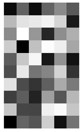
It is 6x10 and uses 600 bytes of disk space.

And this is the second one:

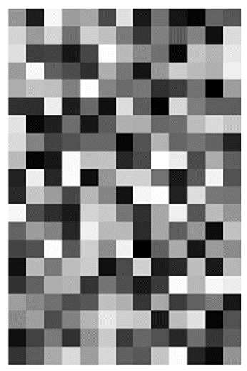
It is 13x20 and uses 1.36KB of disk space.

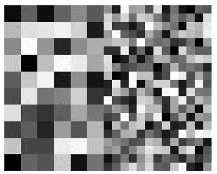
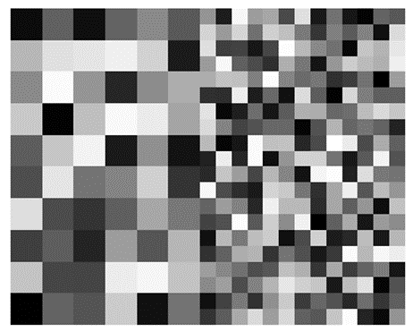
Side-by-side, they look like this:

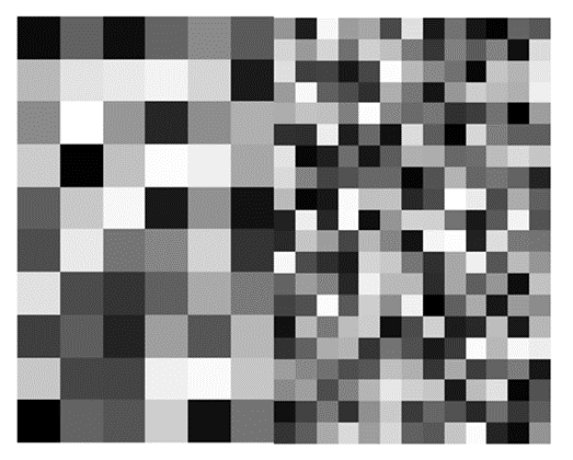
The second raster has a pixel size (5000) that is a half the size of the one of the first raster (10000). They are also slightly misaligned.

Example Task

I want to do some kind of processing that involves both rasters, let’s say, to calculate zonal statistics in this region defined by a 20-sided polygon:

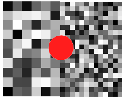
But, in the Zonal Statistics algorithm window, I notice that there is place for only one raster input, and I want the statistics to be calculated for the whole region of the polygon, encompassing parts of both rasters.

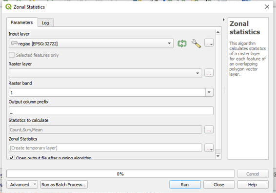
So, yes, we need to mosaic the rasters! (or so I thought)

Mosaicking rasters on QGIS

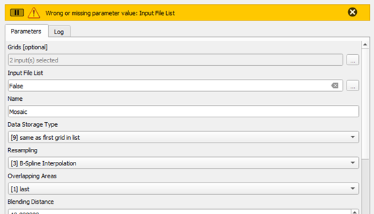
This is my experience mosaicking rasters in this QGIS version (3.26.2). I did not manage to make the algorithms i.image.mosaic from GRASS GIS and Mosaicking from SAGA GIS work smoothly from inside QGIS.

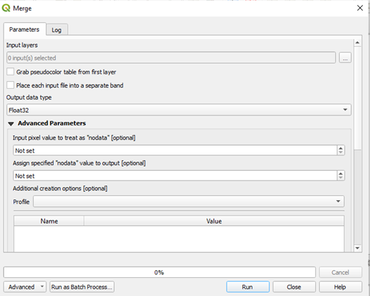
However, the tool “Merge” found in the dropdown menu, in Raster, Miscellaneous, is simple to use and worked well for me.

The resulting raster is:

We can notice that the rasters, previously slightly misaligned, are now perfectly aligned.

If this is good or bad, it depends on your application. Can a small misplacement be accepted for the sake of alignment, or will it have unintended consequences?

Because these are random rasters generated as an example, I accept that, when they align with each other, the second raster also moves up a bit.

Another aspect to notice: in the mosaicked raster, the pixel size is fixed as the one from the most defined raster.

This can be observed in the properties of the generated raster:

Building virtual layers instead

Ok, I showed you how to mosaic rasters. But wasn’t this post about NOT mosaicking rasters?

Yes, let’s build this virtual layer!

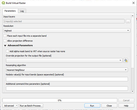
In the processing toolbox, search for the GDAL tool “Build Virtual Raster” (Algorithm ID: gdal:buildvirtualraster).

Select the input rasters and the resolution as “Highest”.

The result is visually very much like the mosaic made with the Merge tool:

The rasters were also automatically aligned and the resulting pixel size is 5000.

ATTENTION: The virtual layer simply references the .tif rasters for a single visualization or for easiness of geoprocessing. If one deletes the original raster files, the virtual layer will stop working!

Use of hard disk memory

The resulting raster generated from mosaicking with the Merge algorithm resulted in an output file of 2.30KB.

The virtual raster file “.vrt” uses 1.80KB, therefore saving hard drive memory.

Opening the virtual layer file, I see:

<VRTDataset rasterXSize="25" rasterYSize="20">
  <SRS dataAxisToSRSAxisMapping="1,2">PROJCS["WGS 84 / UTM zone 22S",GEOGCS["WGS 84",DATUM["WGS_1984",SPHEROID["WGS 84",6378137,298.257223563,AUTHORITY["EPSG","7030"]],AUTHORITY["EPSG","6326"]],PRIMEM["Greenwich",0,AUTHORITY["EPSG","8901"]],UNIT["degree",0.0174532925199433,AUTHORITY["EPSG","9122"]],AUTHORITY["EPSG","4326"]],PROJECTION["Transverse_Mercator"],PARAMETER["latitude_of_origin",0],PARAMETER["central_meridian",-51],PARAMETER["scale_factor",0.9996],PARAMETER["false_easting",500000],PARAMETER["false_northing",10000000],UNIT["metre",1,AUTHORITY["EPSG","9001"]],AXIS["Easting",EAST],AXIS["Northing",NORTH],AUTHORITY["EPSG","32722"]]</SRS>
  <GeoTransform>  3.2483565110000002e+05,  5.0000000000000000e+03,  0.0000000000000000e+00,  6.8163052139999997e+06,  0.0000000000000000e+00, -5.0000000000000000e+03</GeoTransform>
  <VRTRasterBand dataType="Float32" band="1">
    <ColorInterp>Gray</ColorInterp>
    <SimpleSource resampling="nearest">
      <SourceFilename relativeToVRT="1">raster_test_2.tif</SourceFilename>
      <SourceBand>1</SourceBand>
      <SourceProperties RasterXSize="13" RasterYSize="20" DataType="Float32" BlockXSize="13" BlockYSize="20" />
      <SrcRect xOff="0" yOff="0" xSize="12.9451556" ySize="19.9483487200001" />
      <DstRect xOff="12.0548444" yOff="0.0516512799998745" xSize="12.9451556" ySize="19.9483487200001" />
    </SimpleSource>
    <SimpleSource resampling="nearest">
      <SourceFilename relativeToVRT="1">raster_test.tif</SourceFilename>
      <SourceBand>1</SourceBand>
      <SourceProperties RasterXSize="6" RasterYSize="10" DataType="Float32" BlockXSize="6" BlockYSize="10" />
      <SrcRect xOff="0" yOff="0" xSize="6" ySize="10" />
      <DstRect xOff="0" yOff="0" xSize="12" ySize="20" />
    </SimpleSource>
  </VRTRasterBand>
</VRTDataset>

Showing that the virtual layer loads the .tif rasters and displays them as a single layer. The size of the .vrt file seems to be more dependent on the number of raster files composing the virtual layer than on the size/definition of the original layers which compose it.

Zonal Statistics

I executed zonal statistics for both the Virtual and the Merge-generated rasters. It generated the exact same results:

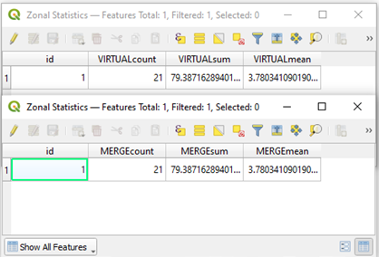
…which is great!

Virtual layers are suited to substitute raster mosaicking for most applications.

Extras

• When would you suggest NOT to use Virtual Layers instead of mosaicking data?

If your data is moved around or recreated with different properties constantly, the virtual layer can fail to load one or more rasters that compose it.

Also, if you need the mosaicked layer as a .tif for something, e.g. to work with it on Python, I don’t suggest using a virtual layer, because it will not generate the needed file.

• Why would you need to visualize two or more rasters together? Why not simply opening them at the same time in your QGIS project?

Ok, but I might need to do some calculations too, such as Zonal Statistics, exemplified in this post.

• 1.80 KB against 2.30 KB is not a large difference at all.

In this case, it’s not, because the used rasters are random, tiny ones, created just for testing purposes. As a test, I joined two large rasters from my PhD research data in a virtual layer, each one is 188 MB, and the resulting “.vrt” file ended up with 1.98 KB. In this case, a lot of storage space was saved.

• Ain’t it obvious that virtual layers are much smaller and the obvious solution for this case?

Perhaps it is, but many people don’t know that virtual layers can be used in basically any calculation and statistic in QGIS.