Fellow researchers and open-source GIS enthusiasts,

Welcome to my blog!

I’d like to start with a disclaimer – I may be a researcher of this very area but that doesn’t mean everything I do or write here will work for you, in your own desktop configurations and package versions. I have no responsibility if you lose data or mess up your installation. I also do not authorize any copies of my content, except for the gists, which are available under the MIT License.

Today, I am going to present a gist that I developed that separates the masking information contained in a Fmask layer into different bands, to be visualized separately. We will visualize it in QGIS, using the Python Console of QGIS, also known as PyQGIS.

This week, I encountered an old frenemy (friend and enemy) of mine on Remote Sensing datasets, the Fmask. This is a masking layer, that usually comes as one of the bands or rasters provided with the original remote sensed product tile that one happen to be downloading. However, this Geotiff very intelligently uses all the bits in a byte, each bit in each byte in each pixel is relative to a different classification, that can be further used, as masks, by us Water Resources or Environmental Engineers and Researchers.

I confess that I find this way of saving the masks much more genial than annoying. That’s the same I think of the grib2 file format. And if it annoys me and others, well, we’re all wrong, because this kind of format saves tons of space! Can you imagine having to download other 6 rasters for each tile, just for the masks? Oof!

Ok, but exactly how is data inside an F Mask stored?

Each information (unrelated to others) is saved in one bit inside the byte, 0 usually means absence of such element, and 1 usually means presence. Example, if a given bit means “snow/ice” and its value in a given pixel is 1, this means that this pixel has snow or ice coverage. This is relevant for remote sensing investigations, because, for many kinds of analyses, this pixel will need to be discarded because it’s reflectance value will be artificially very high for the used bands.

Let’s look into, specifically, the Fmask provided with the product Harmonized Landsat Sentinel, provided by NASA. LP DAAC from NASA has put together a tutorial about basic HLS processing.

Of course, many other NASA products provide Fmask layers or other masks embedded.

For HLS, Table 10 of the HLS user guide gives us information about the content of each bit in the Fmask layer.

A bit of theory

A byte consists of 8 bits, numbered 0 to 7. Each bit is binary, i.e., can be filled with only 0 or 1. This allows the representation of 256 unique values ( $2^8$ ) by each byte. Sure, you can have different ways of storing number information in a byte, such as floats, and so on, but that’s not the point here. This is how most software would read a byte that is consisting of integers, or, more clearly, the information stored in a byte.

This is how QGIS would read (and reads) your bytes that make up for the pixels in Fmasks. By default, it opens the Geotiff of the Fmask and shows you the composed value from the masks provided, in a way that is not necessarily user friendly, unless you are really good in mathematical factorization.

Factorization?

Yes, factorization, if you see that a given pixel of interest has a value of 192 in the F Mask, what does that mean? Would you know, just by looking at it, what masks are in effect, what has been flagged by Fmask, and what has been not? I know I wouldn’t.

An easy to figure out would be to factorize the value 192 in a 2 base. Back to school:

$2^7=128$

is the largest potence of 2 that can be subtracted from 192. Therefore, we should do our number minus 128 and redo this operation for the next largest potence of two possible.

$192 - 128 = 64$

In this case, it is $2^6$.

$2^6=64$

$64 - 64 = 0$

The remainder is already zero, so we don’t need to any further operations.

So, 192 is

$1\cdot128+1\cdot64$

This means that the flagged bits are 128 and 64. 128 is $2^7$ and 64 is $2^6$ . So these are the bits in positions 6 and 7. They are 1, while the other bits are 0. These two bits represent, according to the HLS table, the aerosol quality classification, and, together, mean “High” Aerosol Quality.

Huh, that wasn’t hard at all? Tell me again why did you do a Python code to do this.

Ok, sure! We did it, we factorized 192! But let’s picture a scenario, the tile you downloaded now seems to have like 10 unique bit combinations, each with a different number you’ll have to factorize. And turns out, you just want to the take a peek at the water mask! How can you separate visually the water mask from the other stuff going on there?

If you prefer to do grade school level calculations in your head all the time, by all means keep doing it, I’m just trying to provide a simpler alternative.

How does my Python (PyQGIS) gist work?

It does the factorization inside it, and then saves each information in a separate band in a tif raster. It is made for HLS, but feel free to update it for your preferred dataset.

I’m here for the PyQGIS code gist

This is the gist, hosted on GitHub.

How to use the gist

I wrote a couple of instructions below on how to run the gist.

Define the Fmask raster location

Rasterloc = 'location of my Fmask raster'

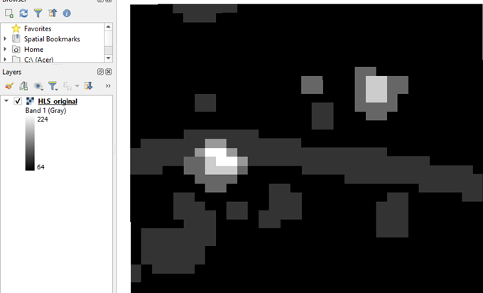
Here is a crop or zoom-in of an original HLS Fmask.

Define the name with which to save your final file

Saveloc ='location to save processed raster'

Run the gist in the Python Console of QGIS

Call the function

New_layer=Fmask_bit_band_separation(rasterloc,saveloc)

Adjust the symbology to see the masks separately or to compose them 3-by-3

After calling the function, you’ll notice a new layer in your layer panel.

For our example, it looks like this:

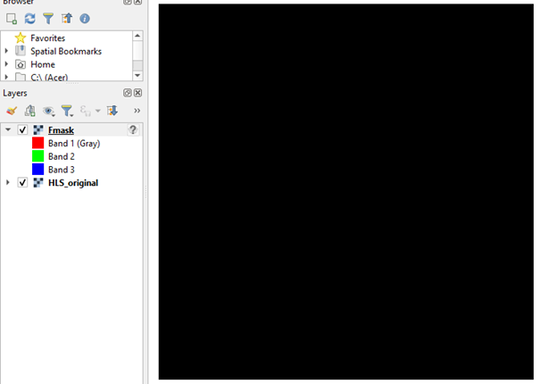
As a multiband raster, its default visualization is RGB, each color representing one of the first 3 bands. The first three bands are all zeros for this case.

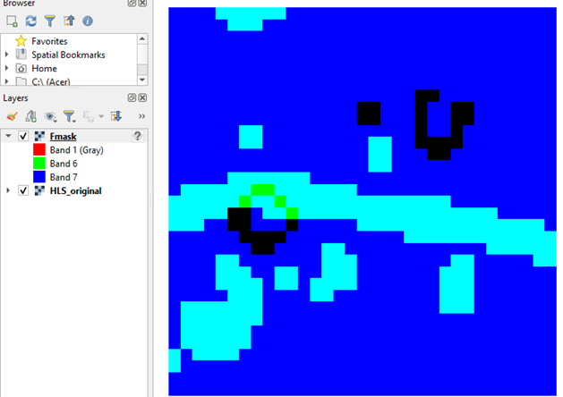
We can change the colors represented by RGB to make the visualization more clear. In this case, I added the bands 6 and 7 to the visualization.

Sometimes it’s best to change the symbology to singleband gray in order to see a mask separately from the others. If we want to see the mask for Water, that is band number 6.

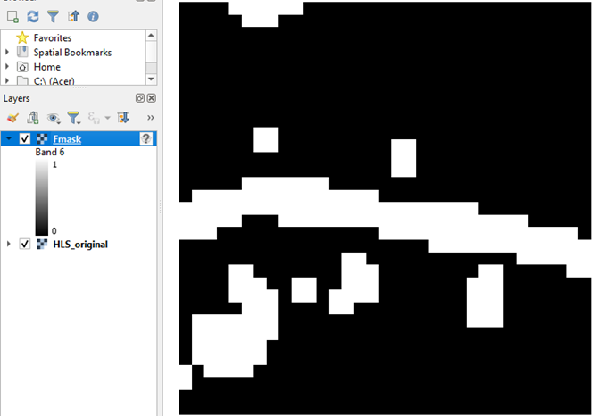
Areas that have value of 1 have Water, and areas that have value 0 have not. This mask is binary and does not convey “degrees of wetness”. In the resulting Water mask, we can clearly see a stream crossing the middle of the raster.

Done!

Extras

• There is a LP DAAC tutorial that teaches how to read Fmask data in Python. Why are you not using their code here?

That is a very useful tutorial, and it did help me deal with Fmask in a NASA project I’m collaborating. However, the QA part of this tutorial teaches how to mask areas of HLS inside a Python code, but not how to save individual outputs of the different bands, nor how to open the resulting raster automatically on QGIS. It could be used as a base, but I chose to make the calculations my own way, from scratch.

• Why is my final Fmask Geotiff much larger than my original?

That is because the original format of the Fmask is optimized to use the minimum amount of storage it can use. When we unravel those single-bit individual masks and save each one in a different band, we are saving each of those bits in a byte. This is a waste of space. Purposeful, since it helps us, researchers, engineers, data analysts, and GIS programmers to understand the data. But yes, it is wasteful from a computational point of view.