Guide to calculate the Vertical Distance to Channel Network (VDCN) step-by-step, tutorial using only open-source GIS software QGIS and SAGA GIS
Fellow researchers and open-source GIS enthusiasts,
Welcome to my blog!
I’d like to start with a disclaimer – I may be a researcher of this very area but that doesn’t mean everything I do or write here will work for you, in your own desktop configurations and package versions. I have no responsibility if you lose data or mess up your installation. I also do not authorize any copies of my content.
Today, the post is about how to generate the raster for Vertical Distance to Channel Network (VDCN) using QGIS Raster Calculator, and SAGA on QGIS or command line interface (CLI), step-by-step.
Vertical Distance to Channel Network (VDCN) is the vertical distance to the interpolated Channel Network, or the river network of the location.
There is a tool on SAGA called “Vertical Distance to Channel Network” that can be used for this matter. The current post is about the possibility to perform the calculations yourself and have more power and control over the process. Or, in some cases, the SAGA tool takes a long time for big spatial data and solutions that can be split in different processes are desirable.
Why generate the Vertical Distance to Channel Network?
VDCN is an important Terrain Attribute that provides information about the approximate depth of the base level flux of a catchment in a point in space. This is useful to know how far the place is from the groundwater, which can be useful for a range of applications in Hydrology, Geomorphology and Natural Hazards studies.
The base level is the level in which the groundwater can be found. Unless measured in field, the base level must be estimated by indirect measurements. If you have actual measurements of the groundwater depth at your site, consistent and spatially distributed, you can simply interpolate your measurements to a raster and this is the vertical distance to the drainage network.
If you don’t have this in situ measurement, you can either go through the steps listed below or employ your tool of choice, one example is “Vertical Distance to Channel Network” from SAGA GIS, that needs the drainage network as an input.
For this tutorial you’ll need:
Your Digital Elevation Model (DEM)
QGIS 3 or superior (Download from qgis.org)
SAGA GIS on QGIS or command line saga_cmd.exe (Download from saga-gis.org – I taught how to use it in this post)
Well, let’s do it. Ready?
- (optional) Reproject the DEM raster
Reproject the raster to a projected cartographic projection (such as UTM), instead of a geographical (lat long). My favourite algorithm for such is gdal Warp. It can be found in QGis 3 on the Processing Toolbox.
- Fill Sinks on your Digital Elevation Model (DEM)
Use your preferred tool to fill the sinks in your DEM. My preferred one is SAGA Sink Removal. On the Prompt, use saga_cmd as (check the post for details on how to use saga_cmd):
saga_cmd ta_preprocessor 2 -DEM input_DEM.tif -DEM_PREPROC DEM_filledsinks.sdat
If your raster is large, this can take some time. On QGIS 3.16, this tool is found on Processing Toolbox, “Fill Sinks”.
- Calculate the Accumulated Flux using a Deterministic 8 (D8) approach
I like using Deterministic approach better for this kind of algorithms, because it generates a single stream instead of a bunch of parallel streams.
3.1 What a D8 Flow Accumulation does, and why is it important to fill sinks before accumulating the flux?
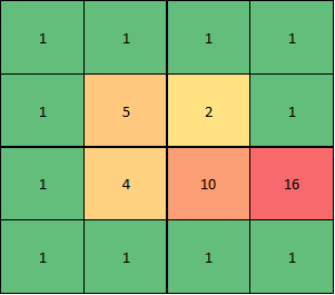
Let’s pretend this is your DEM (the numbers are the elevation values, in meters)
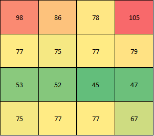
From it, it is easy to see that the channel is in the third line.
To perform the Flow Accumulation, first, the algorithm calculates the direction of the flux, based on the eight possible directions for each point:
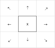
That’s why it’s called D8, abbreviation from Deterministic 8.
The chosen direction is the one with the lowest elevation, except if the elevation of the given cell is lower than that of all the surrounding cells. For our proposed DEM, we can see this occurs in this pixel:
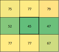
When this happens, we call it a sink. When we perform an algorithm to remove sinks, what we aim to remove is this kind of occurrence, because it creates discontinuities on the flow accumulation.
Why?
Because, based on these 8 possible flow directions, one is chosen, and it is like all the rainfall from the original pixel flows to this other pixel with the lowest elevation.
To accumulate the flux, first, the number of contributing (upslope) cells is accounted. For the example DEM:
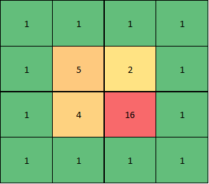
What can we notice here?
The flux is not exiting this region because of the sink. Filling the sink we get a new DEM:

That generates this flow accumulation based on D8 algorithm:
Much better! Now the flux is exiting this part of the DEM, as it is supposed to do.
Some algorithms multiply the number of cells by the area of each cell to calculate the upslope area for each cell.
3.2 Calculating Flow Accumulation
The module Flow Accumulation (Flow Tracing) from SAGA can be used on saga_cmd as:
saga_cmd ta_hydrology 2 -ELEVATION DEM_filledsinks.tif -CAREA flow_accumulation.tif -CAREA_UNIT 0 -METHOD 0
CAREA_UNIT is the unit for accumulating the flux, 0 for the number of cells, and 1, for the uplslope area. If you choose option 0, it is easy to obtain the uplslope area, if you are working with a projection such as UTM, just multiply the flow accumulation in cells by the area of each cell. Let’s say the cell size is 30 m, then the area of each cell is 30*30=900 m². Conversely, if you pick option 1, you can obtain the number of cells by dividing the values by the area of each cell. Both options are OK for calculating VDCN.
Depending on the version of SAGA GIS, CAREA can be FLOW and CAREA_UNIT, FLOW_UNIT.
METHOD indicates the method for performing the calculations. The option 0 is D8, which is my suggestion. But choose other options if you want, you do you!
In QGIS 3.16, the most similar tool is Catchment Area. It does not specify the unit in which the flow will be accumulated, but after a small test, I believe that it is the area (equivalent to option 1 of saga_cmd).
- (optional) Calculate the natural logarithm of the flow accumulation
Your Flow Accumulation output is rather hard to see on QGIS or other geoprocessing software because the scale in which it is represented is linear, but the distribution of the values in your raster approximates more an exponential. To be able to observe the nuances of the flow accumulation raster, I recommend calculating the natural logarithm of it on QGIS Raster Calculator.
Simply use:
ln (“Your Raster”)
and save it to a different name.
And open it in your geoprocessing software and observe it.
- Choose your cutting point
Part of doing this process step-by-step is controlling the small parts of it, such as the threshold for which a cell may be considered part of the channel network.
To do so, I suggest opening the flow accumulation or its logarithm on QGIS and going to Properties of the layer, Symbology. Choose the minimum and maximum accordingly. E.g., if you choose the divide to be between 7 and 8, put 7 as the minimum and 8 as the maximum value. Observe the map. Choose an appropriate number for which the channel network and only the channel network gets highlighted.
Is this your channel network? If it is too comprehensive, choose a higher threshold, if it does not show the higher parts of the watershed, choose a lower threshold. Some people prefer to do this step with the aid of a UAV photo or overlaid satellite image.
When you choose your threshold, keep this number to use it in the next step.
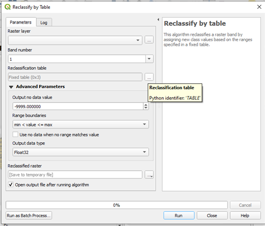
- Reclassify by table
Using QGIS, use Reclassify by table to reclassify your raster using a table.
Search in the Processing Toolbox for Reclassify by Table. Click in the “…” in the right side of Reclassification table to generate your table.
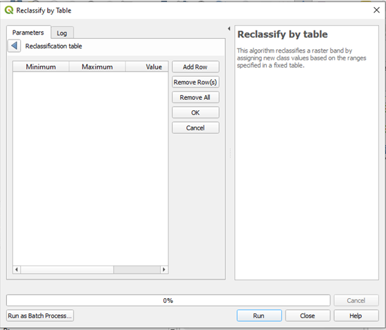 Click in Add Row
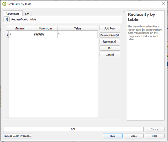
Put your threshold chosen on the previous step as the minimum and a very large number (out of bounds for your raster) as the maximum. These pixels will be replaced by the value 1.
Click OK.
Mark the checkbox “Use no data when no range matches value”. This will make all the rest of your raster become No Data cells. Run the algorithm.
The result will be a raster where the only points that exist are those from your channel network.
- Print elevation values onto the channel network.
To do so, simply multiply the DEM by the raster generated on step 5 using Raster Calculator.
You should get a raster with the elevations over the channel network.
- Interpolate base level
Interpolating the channel network elevation for the rest of the raster, we get a raster with the approximate base level of base flow (subterraneous) based on your given threshold (!). To do that, I switch back to SAGA command line:
saga_cmd grid_spline 5 -GRID channels.tif -TARGET_OUT_GRID interp.tif
for this interpolation, I chose Multilevel B-Spline from Grid Points from SAGA (Multilevel B-Spline Interpolation from raster on QGIS), but you can use any algorithm you like for this interpolation. This one generates a visually smooth raster.
- Calculate the Vertical Distance (to Channel Network)
The last step (probably)!
Calculate the distance to the Channel Network by performing your_DEM.tif – interp.tif in the QGIS Raster Calculator. Save it. Run. Done!
- (optional) Remove the negative values
Some people argue that VDCN should not have negative values, but I believe your final raster has some negative values in a couple of spots. If you are one of these people, reclassify the raster from step 9 in Reclassify by table, but put this in your table:
Minimum: -9999999
Maximum: 0
Value: 0
So it replaces every negative number by zero. Also, remember to uncheck the checkbox “Use no data when no range matches value”.
Luísa Vieira Lucchese
Research Assistant Professor
Research Assistant Professor at University of Pittsburgh